Simulation of Wintertime High Ozone Concentrations in Southwestern Wyoming Using the CALMET CALGRID Modeling System
As summarized in Reed et. al. (2009)[1], the Upper Green River Basin (UGRB), which is located in Sublette County, Wyoming, is bounded by the Wind River Range to the east, the Wyoming Range to the west, the Gros Ventre Range to the north, and bounded by the Uinta Range to the south. These surrounding, significant terrain features effectively create a bowl-like basin that greatly influences the local meteorology relative to the rest of the area. The UGRB is roughly 1,000 meters to 2,000 meters lower than the terrain features to the east and west (WDEQ-AQD 2009)[2].
Within the UGRB, significant development of oil and gas fields has occurred recently. This development has resulted in the release of significant quantities of NOx and VOC emissions, which are both known ozone precursors. Recent monitoring data has indicated elevated ozone concentrations in the late winter that exceed the current National Ambient Air Quality Standards (NAAQS) for 8-hour ozone. As a result of these high concentrations, the WDEQ initiated the Upper Green River Winter Ozone Study (UGWOS) to understand and characterize observed phenomenon.
The 2008 UGWOS final report (ENVIRON 2008)[3] documents the monitoring network and field operations during Intensive Operating Periods (IOPs) that were part of the study during February and March, 2008. The UGWOS field study produced a high quality database of observations for several meteorological parameters as well as ambient measurements of air quality concentrations of ozone precursors in several areas within the Basin. The formulation of the CALMET database has been discussed fully in prior documents (Reed 2009, TRC 2009)[4].
The CALGRID photochemical grid model was run with the above CALMET meteorological database and oil and gas operator-supplied emissions in an effort to replicate the high winter-time ozone concentrations observed at three Federal Reference (FR) ozone-monitoring sites in Sublette Co., WY in February and March 2008. The sites are Daniel, Boulder and Jonah – each within the county and more specifically, the Upper Green River Basin. The ozone monitoring sites are also located close to (Daniel, Boulder) or within (Jonah) active oil and gas field developments, i.e., the Pinedale and Jonah fields. Five full-scale CALGRID runs for the period of February 18-24, 2008, along with several sensitivity and diagnostic analyses, were conducted. The results of this modeling indicate the most sensitivity to VOC speciation and total mass.
EMISSION INVENTORY AND SPECIATON
The Sublette County oil and gas emission inventory was provided by WDEQ and processed by both WDEQ and TRC for CALGRID model input. The emission inventory is comprised of emission sources associated with oil and gas production in Sublette County. The stationary source inventories consist of compressor stations, drill rigs, production sources (heaters, flashing, completions, etc.). Mobile sources were added in Run 5. Generally, the compressor stations and drill rigs are large sources of primary NOx, while the production sources are large sources of VOCs. The VOC emissions in the Basin tend to be of the low reactive variety, but are found at high concentrations near the oil and gas sources. According to the observed canister data, the most abundant high reactive VOCs in the Basin are xylenes (m,p and o) and toluene (ENVIRON 2008)[3], however this can vary by site or time-of-day.
Often, the emission inventory is a source of great uncertainty in photochemical grid modeling, especially the precursor VOC portion. The uncertainty arises from both an observational and modeling point of view, i.e., measurement and/or laboratory issues such as species identification and detection limits contribute to uncertainties as well as the fact that each species has specific reactivity profiles and photolysis parameters for use in modeling. In order to fulfill the chemical mechanisms requirements, the raw VOC emission inventory must be speciated (if only total VOCs provided), or grouped into like-species prior to model input. Given the amount of uncertainty and processing required for the VOC emissions, each of the five model runs represent an additional emission inventory assumption; with each assumption generally considered an improvement or a refinement over the prior analyses.
In order to increase the state of knowledge of the Basin emissions, WDEQ has compiled a detailed inventory of oil and gas sources within Sublette Co. during the months of January through March (the winter inventory). This inventory refines the temporal and spatial resolution of the ozone precursor emissions during the important late winter/early spring months. Information provided by the winter inventory provides monthly hours of operation and emissions for the drill rigs; speciated emissions for specific production activity (e.g., dehys and flashing), wellhead engines, completions and flaring. This inventory was available for winter 2008 and used in the analyses, except Run 1 which used 2007 annual production well data due to time constraints.
The use of a refined inventory, particularly for VOC sources, is expected to provide increased model performance since this is often a model input that has large uncertainty. However, even with speciated VOCs provided by the operators, several iterations and decisions were still required to understand model response and ensure consistency. For instance, some sources or source types had speciated emissions for individual hydrocarbons such as methane through octane (denoted as C1 through C8) or benzene, toluene, ethylbenzene or xylene (BTEX) while others provided only total VOCs. The effect of species treatment was assessed in each of the runs described below. Each run provided additional insights into important model responses and sensitivities to emissions and speciation.
The VOC emissions were processed to conform with the CB-IV chemical mechanism contained within the CALGRID model. CB-IV uses structural-lumping to generalize the representation of chemicals and chemical bonds. Four types of species are present: inorganic species, organic species (e.g. formaldehyde, ethane, and isoprene) that are important to represent explicitly, carbon bond surrogates (PAR = single-bonded carbon atom; OLE = carbon-carbon double bond; ALD2 = carbonyl and adjacent carbon atom), and molecular surrogates (TOL = toluene and other monoalkyl-benzenes; XYL = xylene and other dialkly-benzenes and also triakly-benzenes). Several techniques were used to remap a given emissions inventory to the CB-IV species.
The primary technique uses EPA’s Emission Modeling Clearinghouse Speciation (EMCH) methodology/data. First, a Standard Classification Code (SCC) is assigned for each source in the emissions inventory. Next, the VOC amount is scaled up to TOG (Total Organic Gases, which includes methane and ethane) using a given VOC to TOG scale-up factor lookup table (based on SCC code). Next, the SCC code is matched against a 4 digit Profile code. The Profile code provides the lookup index to a table of mass fractions of the different portion of the TOG, as represented as CB-IV species.
Given the importance of formaldehyde in the area, an optional technique (applied for some sources) replaced the formaldehyde estimated by the SCC code method with the actual formaldehyde value provided in the emissions inventory. This value “overriding” technique preserved the TOG mass by rescaling the non-formaldehyde organic CB-IV species to account for the change in formaldehyde added (or subtracted). For example, if the emission inventory formaldehyde amount for a particular source was 5 lb/hr higher than the SCC method estimation, then the non-formaldehyde species were equally scaled down to remove a total of 5 lb/hr from their emission rates.
Of particular note are Runs 1 and 2 that use the Profile 0000 (SCC 0), which is documented as an “Over All Average” profile, independent of industrial source type. This profile provides a different reactive mixture of CB-IV species than typically found in the SCC codes and attendant Profiles for oil and gas activities. Normally, its corresponding VOC to TOG scale-up factor is 1.0, which assumes that no additional methane and ethane is present (mostly VOCs). In the initial version of the emissions preprocessing program, the VOC to TOG scale-up factors from the SCC-based Profiles (rather than Profile 0000) were used. The SCC-based values are typically larger than 1.0 (e.g. Profile 1001 for Natural Gas Internal Combustion Engines has a VOC to TOG scale-up factor of 10.75). As a result, Profile 0000 runs (Runs 1 and 2) have overestimated VOC emission rates for model input. However, upon review of the total reactive species used for model input, Run 1 has similar values (~5,000 lb/hr) to Runs 3-5 and produced significantly more ozone than Runs 3-5. This is likely due to its more reactive mix of VOCs.
Rather than using the reported total VOC amount, another technique converted each reported organic pollutant (e.g. propane, pentane, benzene, etc.) in the emissions inventory into CB-IV species. Conversion scalars were obtained from Dr. William Carter’s (UC Riverside) “emitdb” database (Carter 2008)[5] which has a comprehensive list of scalars to convert a given organic pollutant into the corresponding lumped species of different chemical mechanisms, including CB-IV. This technique does not make any adjustments or estimations for unknown or missing organic species. If a particular VOC or TOG pollutant is not reported, its value is assumed to be zero.
As discussed above, VOC emissions require substantial processing. Each of the runs below used different emissions inputs, assumptions or processing and are described briefly below. Total emissions are summarized in Table 1.
Table 1. Summary of emission inventory for Runs 1-5:
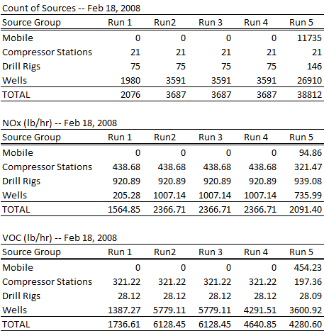
Due to time constraints, CALGRID Run 1 used the 2007 annual well production inventory. The VOC emissions were speciated by default using Profile 0000, which corresponds to SCC 0. Compressor stations were run at their potential to emit values and the drill rigs were run at their reported values.
Run 2 used the 2008 winter inventory for production sources. The VOC emissions were speciated by default using Profile 0000 (SCC 0). Compressor stations were run at their potential to emit values and the drill rigs were run at their reported values.
Run 3 used the 2008 winter inventory and speciated the VOC emissions using respective SCC codes for each source type. Compressor stations were run at their potential to emit values and the drill rigs were run at their reported values.
Run 4 used the 2008 winter inventory and used the operator reported speciation when possible and respective SCC codes for all other sources. Compressor stations were run at their potential to emit values and the drill rigs were run at their reported values.
Run 5 used the 2008 winter inventory and used the operator reported speciation and field-specific speciation when possible and respective SCC codes for all other sources. Compressor stations were changed to reflect their actual emissions and the drill rigs were run at their reported values. Mobile sources were added to the inventory. It is important to note that the number of drill rig and well sources increased in Run 5 since like-drill rigs were not combined into a single source as they were in Runs 1 – 4; and similarly each well source was modeled with its own stack parameters rather than grouped together as a single source as they were in Runs 1 - 4.
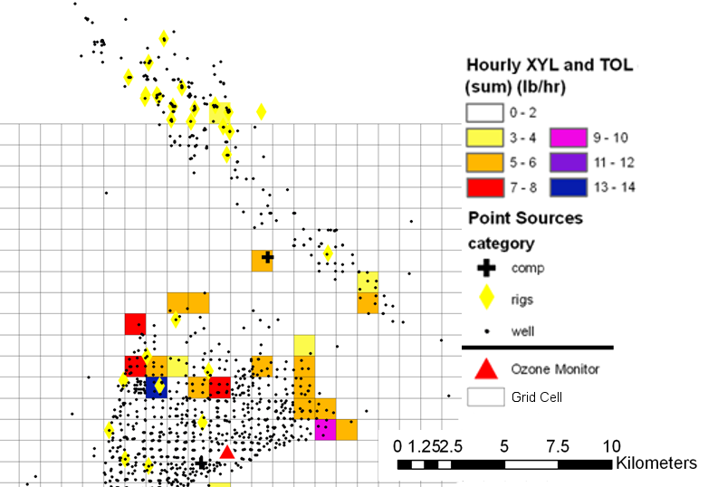
Gridded emissions for Run 5 of key species such as NOx, xylene (XYL) and toluene (TOL) nearby the Jonah federal reference monitors are provided in Figures 1-2. From review of the figures it is evident that the emissions are heterogeneously spread in the Basin with localized areas of high NOx and/or VOC emissions. The heterogeneity of the emissions, when combined with local-scale transport and diffusion under stagnant conditions, increases greatly the complexity of the analysis.
Figure 1. Hourly gridded NOx emissions (lb/hr) near the Jonah Monitor (Run 5):
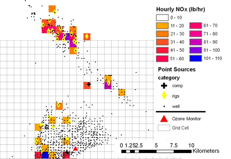
Figure 2. Hourly gridded XYL and TOL emissions (lb/hr) near the Jonah Monitor (Run 5):
SENSITIVITY ANALYSES
Vertical Velocity
Often, large vertical velocities can be found in diagnostic meteorological models such as CALMET in areas of complex terrain or when the observations do not match the initial guess field. As a result, the magnitude of high vertical velocities within the CALMET windfield and their potential effect on CALGRID modeling results has been tracked throughout the project. Vertical velocities within the meteorological data can directly promote the vertical movement of pollutant mass. This vertical movement can result in enhanced dilution (downward movement from the clean layer above the mixing height) or enhanced movement of species outside of the mixed layer from upward movement.
The direct effect of vertical velocity fields has been assessed by running the CALMET model with two different model options related to the vertical velocity: the O’Brien switch ‘on’ and ‘off’. When the O’Brien option is ‘on’, it suppresses (sets equal to 0) the vertical velocity at the top of the modeling domain (and less so in layers below), and adjusts the horizontal winds accordingly so that they are non-divergent. The default value, ‘off’, has been used in the final CALMET windfields and the initial CALGRID assessment, however, the CALGRID model was run using CALMET datasets run with both O’Brien values as sensitivities. No significant difference was seen in the predicted ozone ground level concentrations.
CALMET Version 6
CALMET has been rerun using the latest version of the CALMET (Version: 6.327). This model version has several advantages over the EPA-approved version 5.8 (used in Runs 1-5) such as known bug-fixes and other model options that may address specific technical concerns including the use of local-scale lapse rates rather than domain-scale lapse rates for stability and kinematic calculations, other mixing height options and prognostic model output clouds and relative humidity. In particular, the use of local scale lapse rate calculations available in Version 6 of the model by setting IUPT = -1 (as opposed to a domain-wide lapse rate) were explored for their effect on mixing heights, an important meteorological parameter for ground level ozone concentrations.
Using the Run 5 emissions, the CALGRID model was run with several iterations of CALMET version 6 windfields as summarized in a separate report. No significant model response to any of the CALMET changes were seen, however, these tests may need to be performed periodically in future CALGRID analyses as model performance improves.
CALBOX
Following the consistent underprediction of ozone concentrations (as discussed in Section 4), analyses were performed to try and systematically test known model uncertainties, e.g. the chemical mechanism. The CALGRID CB-IV mechanism was tested by simplifying the model inputs until they represent a box model (i.e., CALBOX) with no horizontal advection (from boundary conditions or sources) or vertical advection (from reservoirs aloft).
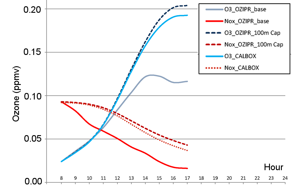
CALBOX was applied to the February 20, 2008 observed morning canister data at Jonah such that it can be compared to the box modeling conducted by ENVIRON using the OZIPRW model updated with CB05 chemistry (ENVIRON 2010)[6]. The models were homogenized by using the same observed data for initial conditions (observed NOx, speciated VOCs and ozone on the morning of February 20, 2008 at Jonah) and preventing entrainment from layers aloft (fixed mixing height for OZIPRW and vertical advection and diffusion turned off for CALBOX), making it easier to assess the differences due to the chemical mechanisms alone. As illustrated in Figure 3, both models produce ozone at concentrations near 200 ppbv. Consistent with other studies, CB05 predicted larger ozone than CB-IV; in this case about 5% larger. These results indicate the CB-IV chemical mechanism has the ability to produce similar ozone concentrations to the CB05 chemical mechanism given the same precursor concentrations. The results of this, and several similar analyses, indicate that CB-IV by itself is likely not the sole reason for underprediction of ozone with CALGRID.
Figure 3. Comparison of CALBOX to OZIPRW using Jonah canister data on February 20, 2008:
CALGRID Version C
The CALGRID model’s transport and diffusion subroutines have also been updated to more recent versions provided by Dr. Robert Yamartino. These updates implement the method that he used in CMAQ (the yamo option). This scheme has several advantages such as the elimination of all transport operator splitting errors and low numerical diffusion along with explicit mass conservation via mixing-ratio (ppmv).
Although this code is still in testing at this time, initial results are similar to those obtained from the previous CALGRID (Version B). The model sub-hourly timestep is now set internally each hour, and fewer than 30 substeps per hour are needed for periods with light wind speeds. This reduces the simulation times. With larger wind speeds, the updated model requires on the order of 30 substeps per hour, which is in line with the results of the sensitivity results obtained with the previous version.
MODEL RESULTS AND ANALYSES
The CALGRID results for Runs 1 through 5 used the above-described model inputs and emissions. The hourly timeseries of model predicted ozone versus observed ozone were plotted at several monitors throughout the Basin, including the Boulder, Daniel and Jonah monitors. The timeseries comparisons were performed for the ‘nearby’ 30 km by 30 km area and at the grid cell of the monitor location (spatially paired). Contours of ozone across the Basin were also produced for review.
Run 1
The 1 hour timeseries plots of layer 1 (10 m) modeled ozone concentrations for the Jonah monitor are provided in Figure 4. The model generally under-predicts at all monitor locations but gets above 100 ppbv at Boulder on February 21 and has 3 straight days in excess of 100 ppbv at the Jonah monitor.
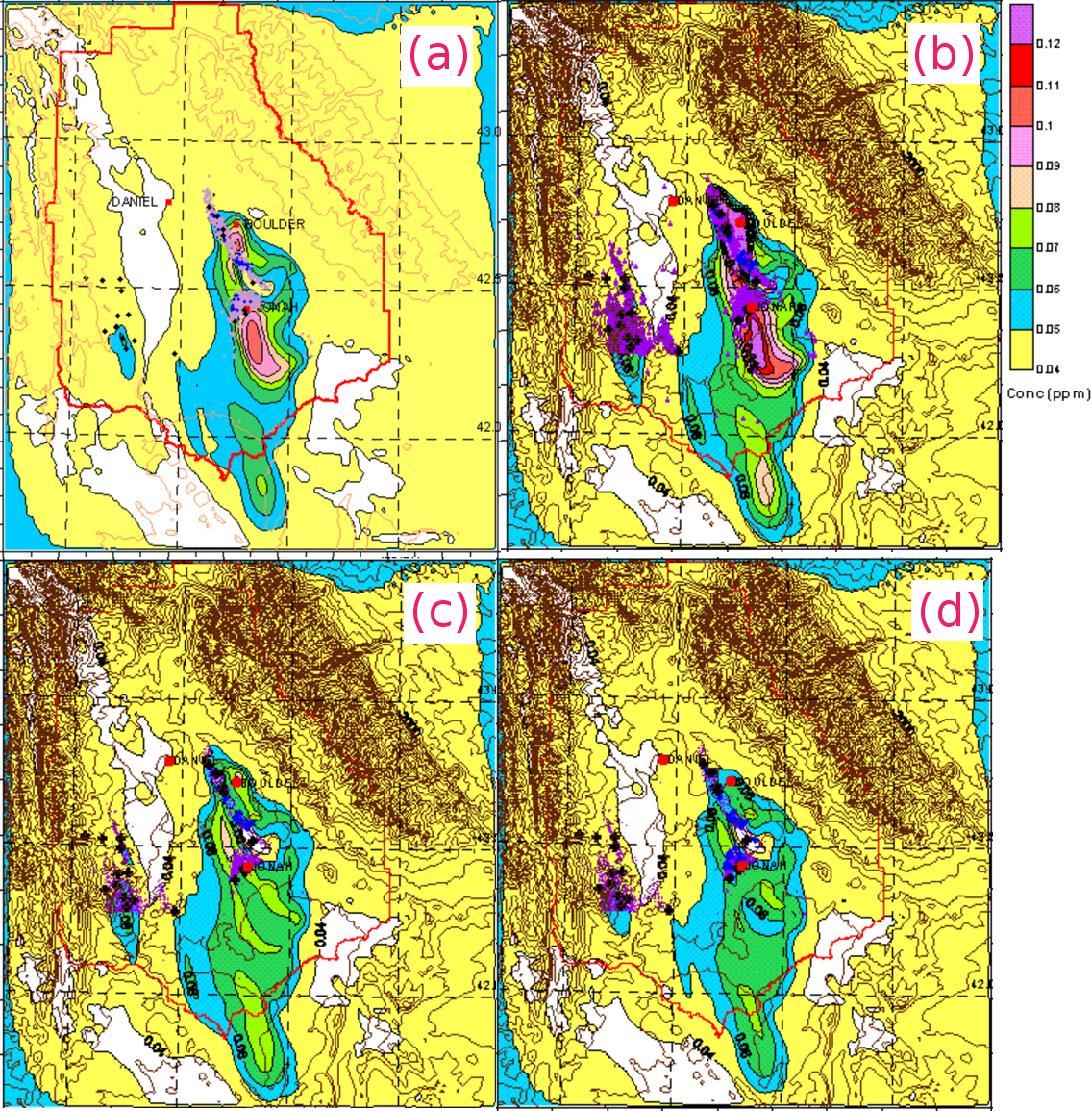
The domain-wide layer 1 ozone contours are provided for 1 pm on February 21, 2008 as shown in Figure 5(a). This period exhibits the typical pattern of winter ozone in Sublette County: stagnant meteorology, low mixing heights and a rapid build-up of hourly ozone as the sun rises. The areas of high ozone are generally small and exhibit very tight spatial gradients within the Basin, which seem to be consistent with aircraft ozone transects across the Basin.
Run 2
The 1 hour timeseries plots of layer 1 (10 m) modeled ozone concentrations are provided for Jonah in Figure 4. The model generally over-predicts at all monitor locations, especially at Boulder and Daniel and has excellent performance at the Jonah monitor.
The domain-wide layer 1 ozone contours are provided for 1 pm on February 21, 2008 as shown in Figure 5(b). The areas of high ozone are similar to that in Run 1, but have a larger magnitude in terms of concentrations and also exhibit very tight spatial gradients within the Basin.
Given the large amount of TOG created during the emission processing procedures relative to the other runs, these results are not considered reliable or representative of the photochemistry occurring within the Basin. At the same time, they can provide useful insights into model response during these conditions, in this case, VOC saturation.
Run 3
The 1 hour timeseries plots of layer 1 (10 m) modeled ozone concentrations are provided for Jonah in Figure 4. The model consistently under-predicts at all monitor locations with decreases of 20 ppbv in ozone at Boulder and Jonah and little change at Daniel when compared to Run 1. Contour plots were not produced for these runs.
Run 4
The 1 hour timeseries plots of layer 1 (10 m) modeled ozone concentrations are provided for Jonah in Figure 4. Similar to Run 3, the model continues to under-predict at all monitor locations with decreases of 20 ppbv in ozone at Boulder and Jonah and little change at Daniel when compared to Run 1.
The domain-wide layer 1 ozone contours are provided for 1 pm on February 21, 2008 as shown in Figure 5(c). The areas of high ozone are similar to that in Run 1, but have a smaller magnitude in terms of concentrations and exhibit weaker spatial gradients within the Basin.
Run 5
The 1 hour timeseries plots of layer 1 (10 m) modeled ozone concentrations are provided for Jonah in Figure 4. The observed ozone concentrations are provided for comparisons. Similar to Runs 3 and 4, the model continues to under-predict at all monitor locations with decreases of 20 ppbv in ozone at Boulder and Jonah and little change at Daniel when compared to Run 1.
The domain-wide layer 1 ozone contours are provided for 1 pm on February 21, 2008 as shown in Figure 5(d). The areas of high ozone are similar to all previous runs, but like Run 4 exhibit weak spatial gradients and consistently lower magnitude concentrations than Runs 1 and 2 and even Run 3.
Figure 4. Comparison of timeseries for Runs 1 to 5 to observed hourly ozone concentrations at Layer 1 (10 m) at Jonah:
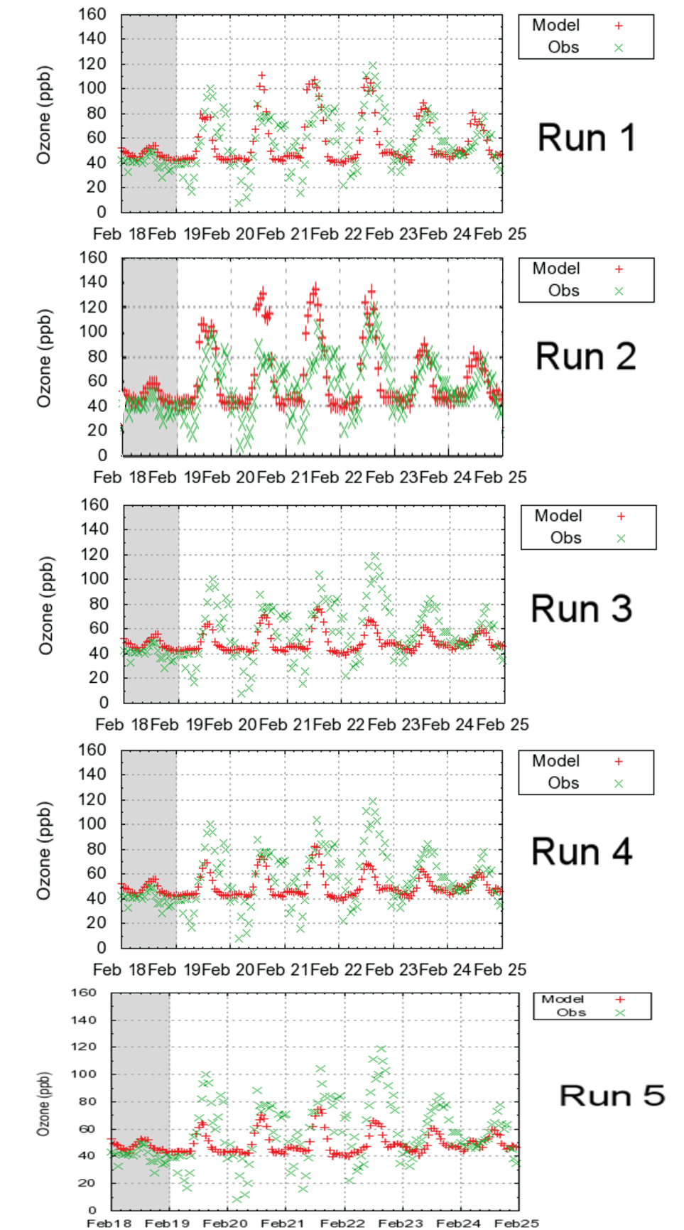
Figure 5. Contours of hourly ozone at Layer 1 (10 m) at Jonah on Feb. 21, 2008 13:00 LST for Run 1 (a), Run 2 (b), Run 4 (c), and Run 5 (d). Red polygon represents ozone non-attainment area. Terrain contours shown as brown lines.
REFERENCES
| [1] | Reed, J.F., Rairigh, K., Newman, M.B., Klausmann, A.M., Scire, J.S. and Hoffnagle, G.F. (2009) “Assessment of CALMET Performance Using In-Situ Data in a Complex Meteorological Environment”, Paper No. 47, A&WMA Guideline on Air Quality Models, Raleigh, North Carolina |
| [2] | WDEQ-AQD. (2009) Technical Support Document I for Recommended 8-Hour Ozone Designation for the Upper Green River Basin, WY. Cheyenne: State of Wyoming. |
| [3] | (1, 2) ENVIRON, T&B Systems Inc., Meteorological Solutions Incorporated. (2008). Final Report 2008 Upper Green River Winter Ozone Study. |
| [4] | TRC. (2009). Upper Green River Winter Ozone Study: CALMET Database Development Phase I. Windsor: TRC. |
| [5] | Carter, W.P.L. (2008). Development of an Improved Chemical Speciation Database for Processing Emissions of Volatile Organic Compounds for Air Quality Models. emitdb.xls database version 2008-10-29. http://www.engr.ucr.edu/~carter/emitdb/ |
| [6] | ENVIRON. (2010). 2008 Winter Ozone Box Model Study. |
AUTHORS
Michael B. Newman1, Jason F. Reed1, Ken Rairigh2, David Strimaitis1, Gale F. Hoffnagle1
- TRC, 21 Griffin Road North, Windsor, CT 06095
- Wyoming Department of Environmental Quality, Air Quality Division, Cheyenne, WY, USA
PUBLISHER NOTES
Paper originally published October 10, 2010 as an extended abstract to accompany a poster presented at the 9th Annual CMAS Conference, Chapel Hill, North Carolina.