PM2.5 Design Concentrations in High Background Regions
Fine particulate matter is frequently becoming the permit limiting air pollutant in modeling compliance demonstrations. High background concentrations of particulate matter less than 2.5 microns in aerodynamic diameter (PM2.5) in many parts of the country present air quality permit modeling challenges for National Ambient Air Quality Standards (NAAQS) compliance demonstrations. An examination of PM2.5 24-hour average background concentrations and AERMOD model predicted concentrations for a proposed facility was conducted to investigate the meteorological events underlying the concentration distributions. Regional transport rather than local sources appeared to dominate the observed fine particulate concentrations. Predicted concentrations from the proposed source were strongly influenced by the complex terrain setting of the facility. High predicted concentrations did not temporally correspond to high observed concentrations; however, it is not fully protective of NAAQS to evaluate only high predicted concentration events. High observed concentration events played a more significant role in establishing the design concentration. Further, EPA’s “Guideline on Air Quality Models” approach for determining background concentrations may not be adequately protective of the NAAQS. For this reason, it was necessary to develop an alternative compliance demonstration approach and obtain regulatory agency buy-in on the technique.
INTRODUCTION
Air quality dispersion modeling is used to predict ambient air concentrations of pollutants emitted by a variety of sources. To calculate the total ambient air concentration, modeled concentrations attributable to modeled local sources must be summed with the representative background pollutant concentration. The background concentration represents the contribution from all other sources not modeled, which may include distant and/or small anthropogenic sources as well as naturally occurring atmospheric concentrations of the pollutant. This paper explores methods of determining 24-hour average background concentrations for PM2.5 that are protective of ambient air quality standards while still permitting environmentally responsible projects.
Typically, background air quality concentrations are derived from historical air quality monitoring data, which tend to be log normally distributed. In this case, the proposed source is located in Connecticut and the Connecticut Department of Environmental Protection (CTDEP) specifies that the initial PM2.5 background concentration (i.e., the design value) be determined as the average of the yearly 98th percentile 24-hour concentrations measured over the last three years of available data. Generally, the data are averaged for the nearest three monitoring sites as shown in Table 1. The background concentration is added to the highest eighth high (H8H) modeled concentration to determine NAAQS compliance. This approach is statistically incorrect, since log normal distributions are not additive, although some authors have suggested approximations for the summations.[1] Note that the average background concentration yields only 2 µg/m3 available for the source impact to remain below the NAAQS. Unfortunately, multisource modeling predicted H8H concentrations exceeding 9 µg/m3, and thus further analyses were required to demonstrate compliance.
Table 1. Design value monitored background concentrations:
| PM2.5 Design Values (2004-2006) | ||
|---|---|---|
| Monitor | 24-Hour Average (µg/m3) | Distance to Source |
| East Hartford | 32 | 26 km south |
| New Haven | 33 | 36 km northeast |
| Waterbury | 33 | 37 km east |
| Regional Average | 33 | |
| NAAQS | 35 | |
APPROACH
The U.S. Environmental Protection Agency (EPA) “Guideline on Air Quality Models,”[2] Section 8.2, discusses the use of monitored air quality data to incorporate the background concentration into the total predicted ambient concentration.
The Guideline states:
“Use air quality data collected in the vicinity of the source to determine the background concentration for the averaging times of concern. Determine the mean background concentration at each monitor by excluding values when the source in question is impacting the monitor. The mean annual background is the average of the annual concentrations so determined at each monitor. For shorter averaging periods, the meteorological conditions accompanying the concentrations of concern should be identified. Concentrations for meteorological conditions of concern, at monitors not impacted by the source in question, should be averaged for each separate averaging time to determine the average background value. Monitoring sites inside a 90° sector downwind of the source may be used to determine the area of impact. One hour concentrations may be added and averaged to determine longer averaging periods.”
Thus, the Guideline provides an approach based on average monitored concentrations to determine the appropriate background concentrations based on concurrent meteorological conditions.
Further, the CTDEP Interim PM2.5 New Source Review Modeling Policy and Procedures[3] (August 21, 2007) states:
“CTDEP may allow an applicant to define background values that are less than the observed design values, provided the applicant provides sound technical reasoning for such an approach (e.g., a directional-specific analysis of monitored levels).”
Thus, both the Guideline and CTDEP’s Interim Procedures provide guidance to determine the appropriate background concentrations based on concurrent meteorological conditions or other “sound technical reasoning.”
The approach used to derive a representative background PM2.5 concentration included the following steps:
- The PM2.5 data from the three closest air quality monitoring stations were reviewed together with the concurrent meteorology.
- Air quality dispersion modeling was conducted to identify the meteorological conditions of interest that are associated with the maximum predicted PM2.5 impacts.
- The monitored concentrations corresponding to the conditions of interest were identified and the appropriate background determined.
OBSERVED CONCENTRATIONS
Air quality dispersion modeling using off-site, National Weather Service (NWS) data is generally performed using five years of meteorological input data to obtain climatologically representative concentration predictions. In order to provide a complete view of the background air quality concentrations during the modeling period, meteorological data and monitored PM2.5 concentrations from the three sites were reviewed for the entire modeling period, 2002-2006.
CTDEP operated the PM2.5 monitoring stations in the region during the 2002-2006 time period. These included Federal Reference Method (FRM) monitoring as well as two sites equipped with Beta Attenuation Monitors (BAM). Table 2 summarizes the data periods and monitor types available at the CTDEP sites in the area. All of the listed monitors continued operating through the end of 2006, but some came on-line at various times during the period. The East Hartford FRM site collected daily filter samples. The other primary FRM sites, the New Haven Agricultural Station and the Waterbury site collected data on an every third day basis. A collocated FRM filter monitor at Waterbury collected data every sixth day.
Table 2. Monitoring period of record:
| Station | Monitor Type | Start Date | Number of Observations* | Montitoring Frequency |
|---|---|---|---|---|
| East Hartford | FRM | 1/1/2002 | 1606 | Daily |
| East Hartford | BAM | 5/17/2004 | 938 | Daily |
| East Hartford | Combined | 1/1/2002 | 1710 | Daily |
| New Haven Ag Stn | FRM | 4/3/2003 | 422 | 3rd Day |
| Waterbury | FRM 1 | 1/2/2002 | 570 | 3rd Day |
| Waterbury | FRM 2 | 1/2/2002 | 290 | 6th Day |
| Waterbury | BAM | 6/19/2003 | 1247 | Daily |
| Waterbury | Combined | 1/2/2002 | 1433 | |
| All Monitors | Combined | 1774 |
*Total possible daily observations 2002-2006 = 1826
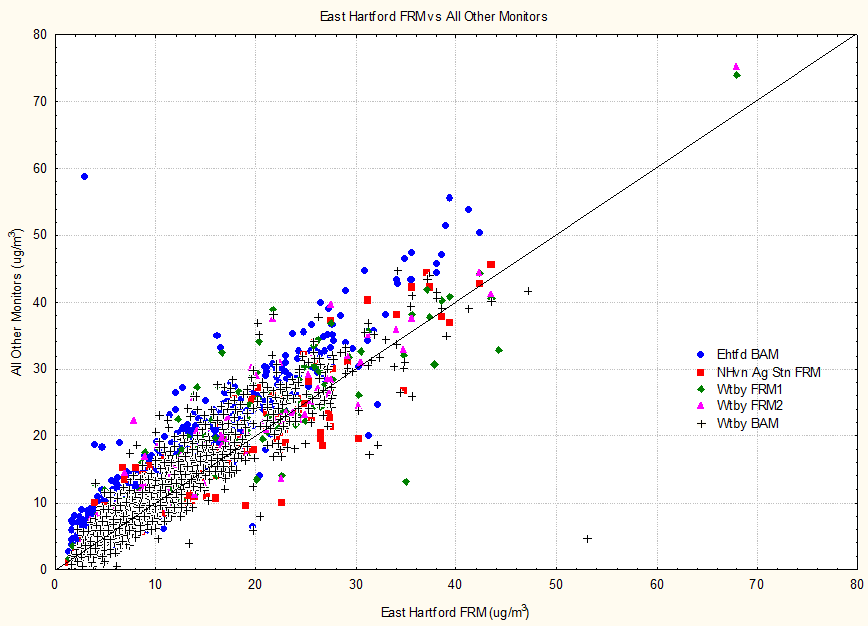
Figure 1 shows concentrations from all other monitors versus the East Hartford FRM. The data track reasonably well with only two obvious significant outliers, both in the BAM data. This figure suggests that daily PM2.5 concentrations at all the sites are dominated by regional influences, since they all track up and down together, with some scatter due to local sources and instrument noise.
Figure 1. East Hartford FRM vs. All Other Monitored Daily PM2.5 Concentrations (µg/m3):
In order to have the most complete record of daily concentrations at each of the three monitoring locations, the data for each day at each site were combined. To generate the combined datasets, the FRM data were selected preferentially and the BAM data were “filled-in” on days when the FRM data were unavailable. In accordance with the “Interpretation of the National Ambient Air Quality Standards for PM2.5,”[4] the two collocated FRM observations from Waterbury were averaged when both were present. This procedure resulted in at least one background concentration observation on 1,774 days out of the 1,826 days (> 97 percent) in the five year modeling period.
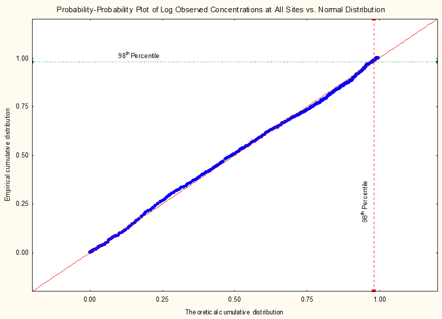
Figure 2 shows that the observed data for all years from all three stations combined are log-normally distributed and that the 98th percentile of the log-normal fitted distribution is representative of the 98th percentile of the observed data at all sites.
Figure 2. Log Probability Plot for All Stations Combined:
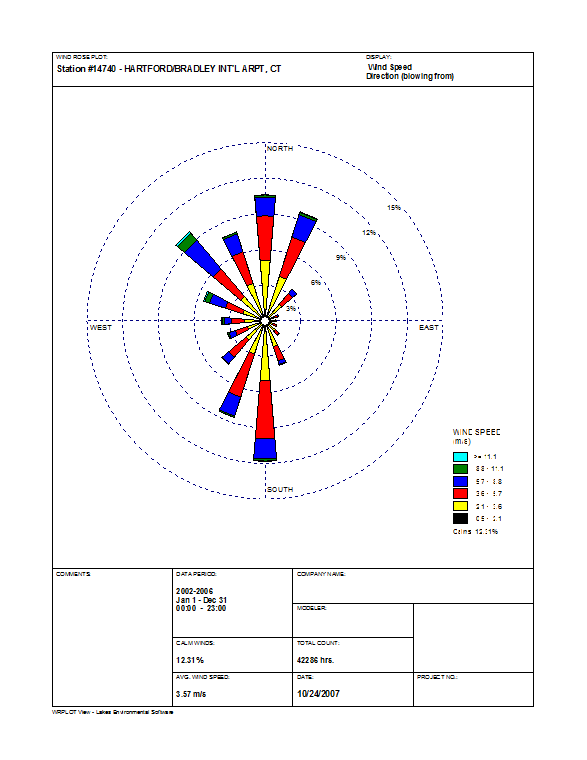
The closest NWS station that collects the meteorological data used for dispersion modeling is at Bradley Airport, approximately 26 miles north of the project site. A wind rose for the five years of modeled hourly meteorological data (2002-2006) from the Bradley Airport NWS station (BDL) is presented in Figure 3.
Figure 3. Bradley Airport Windrose 2002-2006:
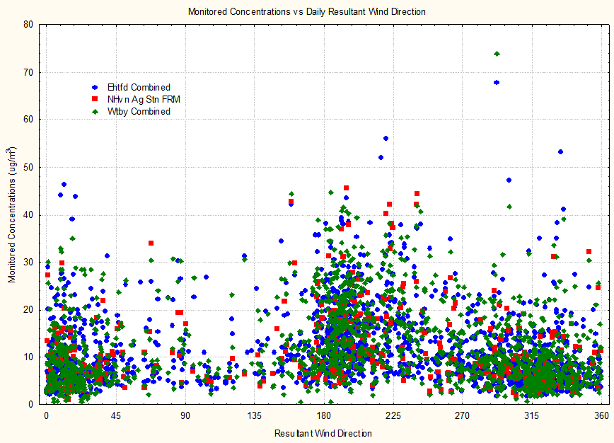
Monitored concentrations were compared to the daily resultant wind direction, the daily average wind speed and the wind direction persistence. The most visible correspondence was between monitored concentrations and resultant wind directions. Figure 4 presents the PM2.5 monitored concentrations for the combined data sets at the three selected sites versus the daily resultant wind direction from Bradley. The southwest wind quadrant has the most monitored concentrations that are greater than 20 µg/m3. This is indicative of transport of polluted air from urban areas to the southwest of Connecticut. The highest frequency of monitored concentrations less than 10 µg/m3 is with winds from the northern directions, reflecting cleaner air advection from the north.
Figure 4. Monitored Concentration vs. Daily Resultant Wind Direction:
PREDICTED CONCENTRATIONS
To determine predicted source contributions, EPA’s AERMOD[5] dispersion model was run. AERMOD uses hourly observed meteorological data, in this case hourly data from Bradley Airport to predict 24-hour average concentrations at an array of receptors surrounding the modeled sources.
The AERMOD model was run for the period 2002-2006 to identify the meteorological conditions of interest leading to high predicted concentrations from all NAAQS sources combined. The pattern of the predicted eighth high 24-hour average concentrations over the three consecutive worst-case years at each receptor, as well as the location of the three year average H8H predicted concentration are presented in Figure 5. The concentrations shown on this figure are the averages of the eighth highest concentrations at each receptor for the three highest consecutive years out of the five years modeled or, in other words, the isopleths for the controlling predicted concentrations for all sources in the multi-source inventory. The high AERMOD predicted 24-hour average concentrations occur on the nearest elevated terrain southeast of the project site. This direction also corresponds to high wind direction frequency as indicated by the Bradley Airport wind rose (Figure 3). Note that the highest predicted PM2.5 concentrations are a small fraction of the highest observed concentrations.
Figure 5. Model Predicted 8th Highest 24-hour PM2.5 Impacts:
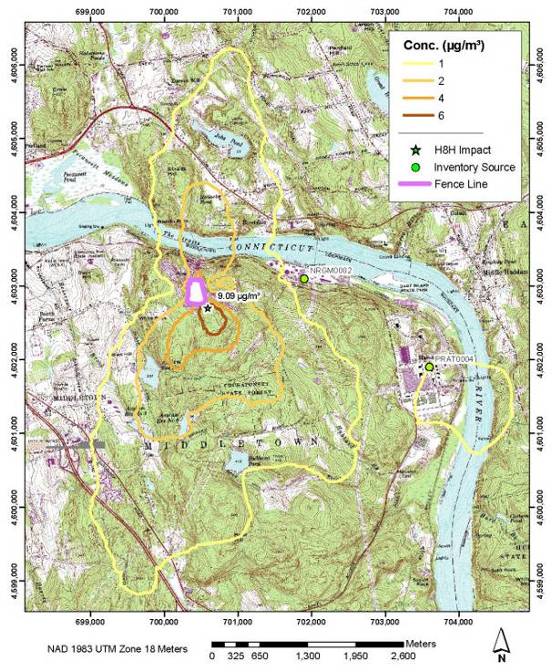
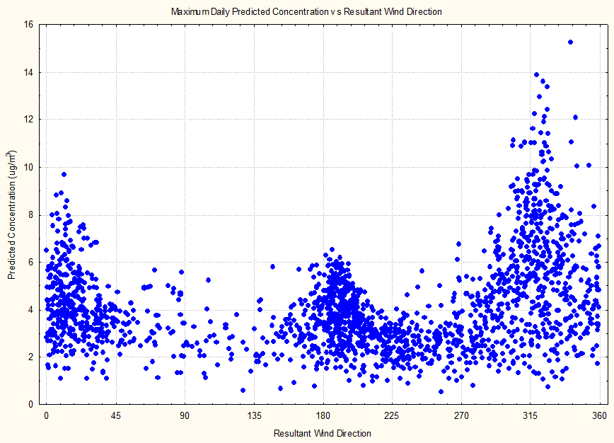
Figure 6 shows the pattern of the resultant 24-hour wind directions versus the highest daily predicted concentrations from all sources in the NAAQS inventory. Figure 6 shows that wind directions from approximately 300 to 360 degrees cause the highest predicted concentrations, with resulting maximum concentration impacts to the southeast or south of the proposed facility. In contrast to Figure 6, Figure 4 shows that the high observed concentrations tend to be clustered within the 180 to 225 degree wind directions, which are just the opposite of the wind directions associated with the highest predicted concentrations.
Figure 6. Maximum Daily Predicted Concentration vs. Resultant Wind Direction:
Given both the federal and state recommendations for refined background concentrations, and the demonstrated tendency for high predicted concentrations in general and the controlling concentration in particular to occur with northwest winds, the average observed 24-hour average PM2.5 concentrations from the closest three monitoring stations have been calculated as presented in Table 4. As expected for log-normal distributions, the mean is higher than the geometric mean or the median, which are better statistical indicators of central tendency for a log–normal distribution. Thus, the mean background concentration is a conservative indicator of the background concentration.
Table 4. Background concentrations by meteorological condition:
| 24-Hour Background Concentration (µg/m3) | ||||
|---|---|---|---|---|
| Valid N | Mean | Geometric Mean | Median | |
| All Observed | 1774 | 12 | 10 | 9 |
| Wind Direction 300-360 | 455 | 8 | 7 | 7 |
EPA conservatively recommends using the mean concentration for the background, which is biased high in the sense that for most days the actual background will be lower than the mean. It is obvious from the data presented and discussed above that the background concentrations are wind direction dependent, thus it would be overly conservative to calculate a total potential ambient concentration based on the sum of the 98th percentile modeled and monitored concentrations if more representative total concentrations can be calculated by summarizing the background concentrations expected during periods of maximum modeled impacts. From Table 4, the appropriate mean background concentration for the days with the maximum modeled AERMOD concentrations (which are associated with wind directions from 300 to 360 degrees) is 8 µg/m3. However, this background concentration may not be conservative for other days when the modeled concentrations are smaller since the modeled impact is only a small part of the total concentration, which is dominated by the background. Although this approach complies with EPA’s Modeling Guideline technique for determining background concentrations, CTDEP would not accept the directionally dependant mean background concentration as appropriate for the NAAQS compliance demonstration.
DAILY COMBINED OBSERVED AND PREDICTED CONCENTRATIONS
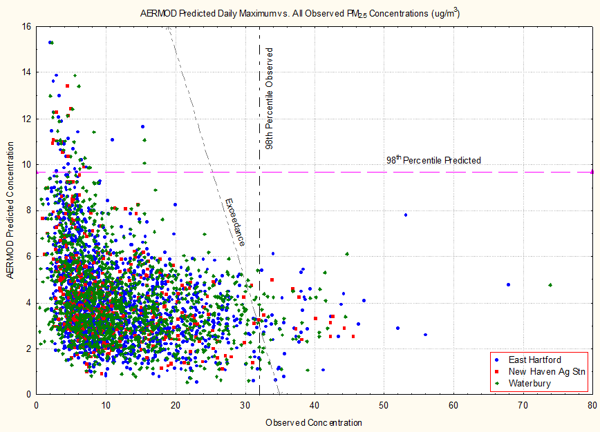
Figure 7 shows the coincidence of the highest daily AERMOD-predicted concentrations anywhere on the receptor array and the monitor-observed concentrations over all sites and years. The 98th percentile observed and predicted concentrations are noted as vertical and horizontal lines on the graph. Predicted exceedances of the 24-hour standard (observed + predicted > 35 µg/m3) are indicated to the right of the diagonal line in the figure. Note that high predicted concentrations (those above the 98th percentile prediction line) tend to occur with low observed concentrations and vice versa. There is a statistically significant negative correlation (r ≈ -0.31) between the observed and predicted concentrations, showing that high predicted concentrations tend to occur with low observed concentrations. This is consistent with the analyses provided above which show the meteorological conditions that lead to the greater than 98th percentile predicted concentrations are not the same as the conditions that lead to the greater than 98th percentile observed concentrations (e.g., north winds lead to high predicted concentrations but generally low observed concentrations, while southwest winds lead to lower predicted concentrations but frequently higher observed concentrations). Viewing Figure 7, it is clear that there are no cases when observed and predicted concentrations are both greater than the 98th percentiles (i.e., there are no points in the upper right-hand quadrant of the figure). This null set corresponds to the generally followed compliance demonstration approach of adding together the 98th percentile observed and the 98th percentile predicted to determine the total concentration for comparison to the NAAQS, even though these two events are unlikely to occur together.
Figure 7. Highest Daily Predicted Concentrations vs. Observed Concentrations at All Sites (µg/m3):
If the occurrence of the predicted and observed peak concentrations is considered to be independent of one another, then the probability of their joint occurrence can be calculated as the product of the frequency of their occurrences. There is a 4 in 10,000 (0.02 X 0.02) chance that the 98th percentile or higher predicted value will occur on the same day as the 98th percentile or higher observed value. Actually, the probability is even less since the predicted and observed concentrations are negatively correlated. This situation corresponds to the upper right-hand region of Figure 7 (both distributions ≥ 98th percentile) and, not surprisingly, there are no occurrences in this very low probability region. Stated differently, there is a 9,996 in 10,000 chance that the observed value corresponding to the 98th percentile predicted value will be less than the 98th percentile observed value.
The preceding situation is similar to the current regulatory scheme using the 98th percentile predicted and the 98th percentile observed concentrations to predict the total concentration. The expected number of days with concentrations greater than this value over a three-year compliance period is 0.4 days. Note that, assuming all years have the same distribution of concentrations, there could be 23 exceedance days before a violation occurs, which is a large safety margin of predicted exceedance days.
While this analysis shows that the current regulatory scheme is very conservative and that the 98th percentile or higher observed and predicted concentrations are very unlikely to occur simultaneously, unfortunately, to the best of our knowledge, there is no way of adding two log–normal distributions together (i.e., the observed background and the model predicted concentrations) and mathematically determining the resulting distribution. Therefore, rather than combining the distributions, AERMOD modeling was conducted and the daily observed background concentrations were added to the daily predicted concentrations at each receptor to predict the total concentration on each day.
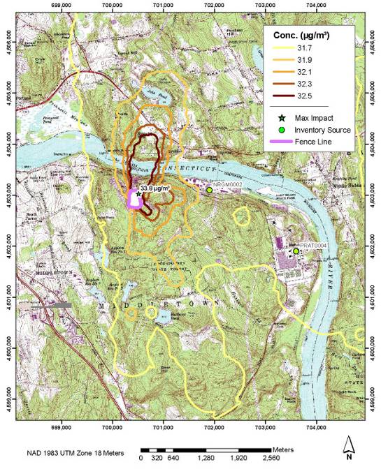
AERMOD was run to predict the impacts of all sources in the NAAQS inventory for the project and the daily background was added to the daily predicted concentrations at all receptor locations. The resulting concentration files were subsequently analyzed to find the highest three-consecutive-year average of eighth high predicted concentrations over all receptors for all modeling years. Figure 8 shows the resulting eighth highest combined daily predicted plus daily background concentrations. The isopleths are for the eighth high concentration at each receptor for consecutive three-year block averages and the maximum concentration (33.8 µg/m3) shown is the overall H8H daily predicted plus background value, which occurred in the years 2003 through 2005. Comparing this with the model predicted concentrations shown in Figure 5 (with high concentrations to the south), it becomes clear that the model predicted concentrations do not drive the total predicted concentration analysis, but that the daily background concentrations (which are highest during southwest winds) do.
Figure 8. Total Model-Predicted Plus Background 8th Highest 24-Hour PM2.5 Concentrations:
The relationship between the daily average background concentrations and the model predicted concentrations is illustrated by showing the time series of both. Figure 9 presents an example of both the daily average monitored concentration and the predicted concentration for 2003 at the controlling receptor location shown in Figure 8 for the combined predicted concentrations and monitored background concentrations. The monitored concentrations (shown in brown) are the daily average of the data available from all three monitoring sites. All missing monitored concentrations (52 days out of 1,826 in the modeling period) were filled with the mean monitored daily PM2.5 concentration of 11.8 µg/m3. The contribution from all NAAQS modeled sources are shown as the AERMOD-predicted green portion of the bars. The concentrations attributable to the modeled local sources are small fractions of the total concentrations. The green dashed line on the figure is the 35 µg/m3 24-hour PM2.5 NAAQS concentration.
Figure 9. Time Series of 2003 Observed and Predicted Concentrations:
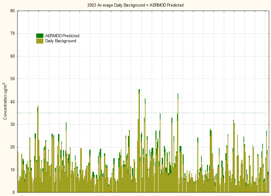
The overall 24-hour average H8H PM2.5 concentration found by combining the daily predicted concentrations with the daily average background concentration is 33.8 µg/m3 based on the three-years of 2003 through 2005, as shown in Figure 8. As discussed above, the background concentration is generally low but occasionally spikes up, sometimes above the 35 µg/m3 concentration level. Examining the figure, it is clear that the EPA Modeling Guideline background approach of using the mean monitored concentrations of 8 to 12 µg/m3 as shown in Table 4 will not yield conservative total predictions.
SUMMARY
Appropriate 24-hour average PM2.5 background concentrations have been derived for modeling analyses based on modeling guidance and concurrent meteorological, air quality modeling and air quality monitoring data. An approach was demonstrated based on an analysis of the monitored and modeled concentrations. It was shown that modeled peak concentrations do not occur simultaneously with high observed background concentrations. The unlikely chance of high background concentrations corresponding to high predicted concentrations is borne out by comparing the actual concurrence of the predicted and observed concentrations. This approach calls for combining the daily predicted PM2.5 concentrations at all model receptors with the daily average observed concentrations from the nearest three monitoring locations. Following the addition of the predicted and observed concentrations, the resulting total concentration files are analyzed to find the average of the H8H total concentration over three consecutive years. This average H8H concentration is compared to the 24-hour PM2.5 NAAQS to demonstrate compliance.
REFERENCES
| [1] | Wu, J, Mehta, N and. Zhang, J., http://www.merl.com/papers/docs/TR2005-099.pdf, accessed (April 2008). |
| [2] | Federal Register, Vol. 70, No. 216, pgs. 68218-68261, November 9, 2005. |
| [3] | CTDEP, CTDEP Interim PM2.5 New Source Review Modeling Policy and Procedures , August 21, 2007. |
| [4] | 40CFR50, Appendix N, “Interpretation of the National Ambient Air Quality Standards for PM2.5.” |
| [5] | http://www.epa.gov/scram001/dispersionprefrec.htm#aermod (accessed February 2008). |
KEYWORDS
MODELING, PM2.5, BACKGROUND, DESIGN CONCENTRATIONS
AUTHORS
Douglas R. Murray, CCM; Michael K. Anderson; QEP, Michael B. Newman, PE; Dana L. Lowes
TRC, 21 Griffin Road North, Windsor, CT 06095
PUBLISHER NOTES
Paper originally published June 24, 2008 as Paper 344 at the 101st Annual Meeting of the Air and Waste Management Association, Portland, Oregon.